A Brief Introduction to Deep Learning
Following a conceptual progression: network structure, gradient descent, embedding vectors, Transformer, attention mechanisms, and MLP fact storage.
Introduction#
This article mainly covers: fully connected networks, backpropagation, Transformers, attention mechanisms, and MLP fact storage.
How do embedding vectors come about? Why aren’t fully connected networks enough? What problem does the Transformer actually solve?
Following a conceptual progression: network structure → learning algorithm → embedding representation → architecture evolution → attention and knowledge storage.
Prerequisites: A basic understanding of matrix multiplication and derivatives. If you’re starting from absolute zero, I recommend watching the original 3Blue1Brown videos first before reading this.
Neural Network Structure#
The Handwritten Digit Recognition Problem#
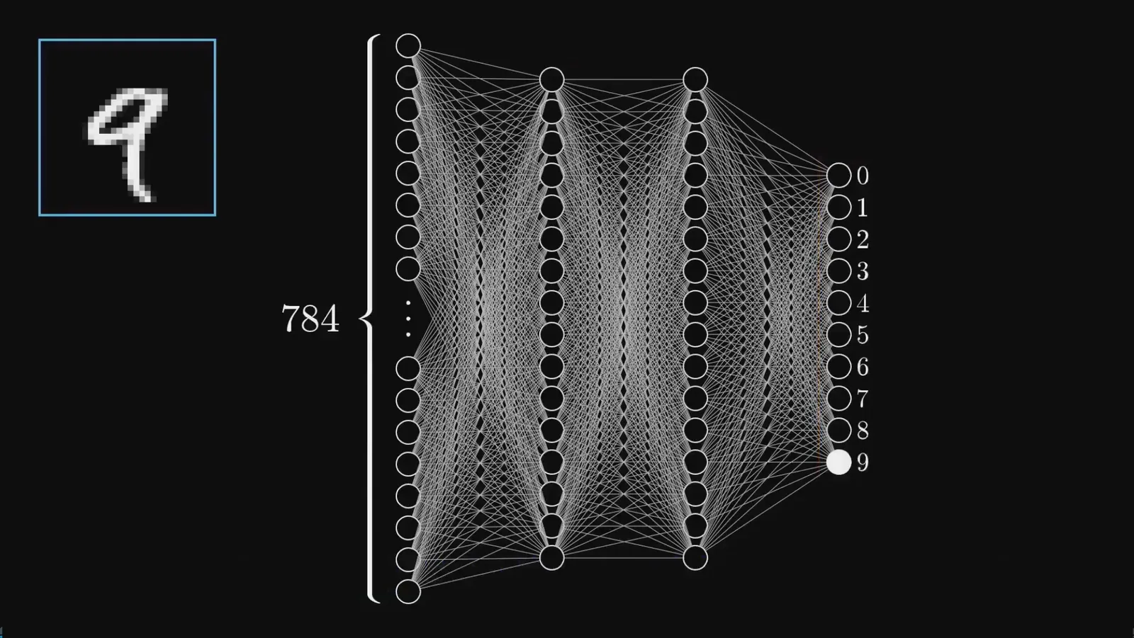
The MNIST dataset is a classic introductory task in deep learning. The input is a 28×28 pixel grayscale image, each pixel represented by a number from 0 (pure black) to 1 (pure white), totaling 784 numbers. The output is a label from 0 to 9 — which digit is written in the image.
Solving this problem with traditional programming is nearly impossible. The digit “4” can be written with an open top or a closed one; “7” can have a crossbar or not. There’s no set of if-else rules that can cover all the variations. Yet the human brain does this effortlessly, without even thinking. Neural networks start from mimicking this biological structure — using layered combinations of many simple units to approximate complex input-output mappings.
Neurons and Network Structure#
A “neuron” in a neural network is far simpler than a biological neuron. It does just one thing: holds a number between 0 and 1, called its activation. 0 means completely silent, 1 means maximally excited. All information in the network flows through these numbers.
Building a concrete network to solve the handwritten digit problem:
| Layer | Neurons | Design Intent |
|---|---|---|
| Input Layer | 784 (28×28) | Each neuron corresponds to a pixel’s grayscale value |
| Hidden Layer 1 | 16 | Detect small-scale edges, short lines, arcs |
| Hidden Layer 2 | 16 | Combine edges, detect components like circles and vertical lines |
| Output Layer | 10 | Each represents digits 0–9, the highest activation is the network’s judgment |
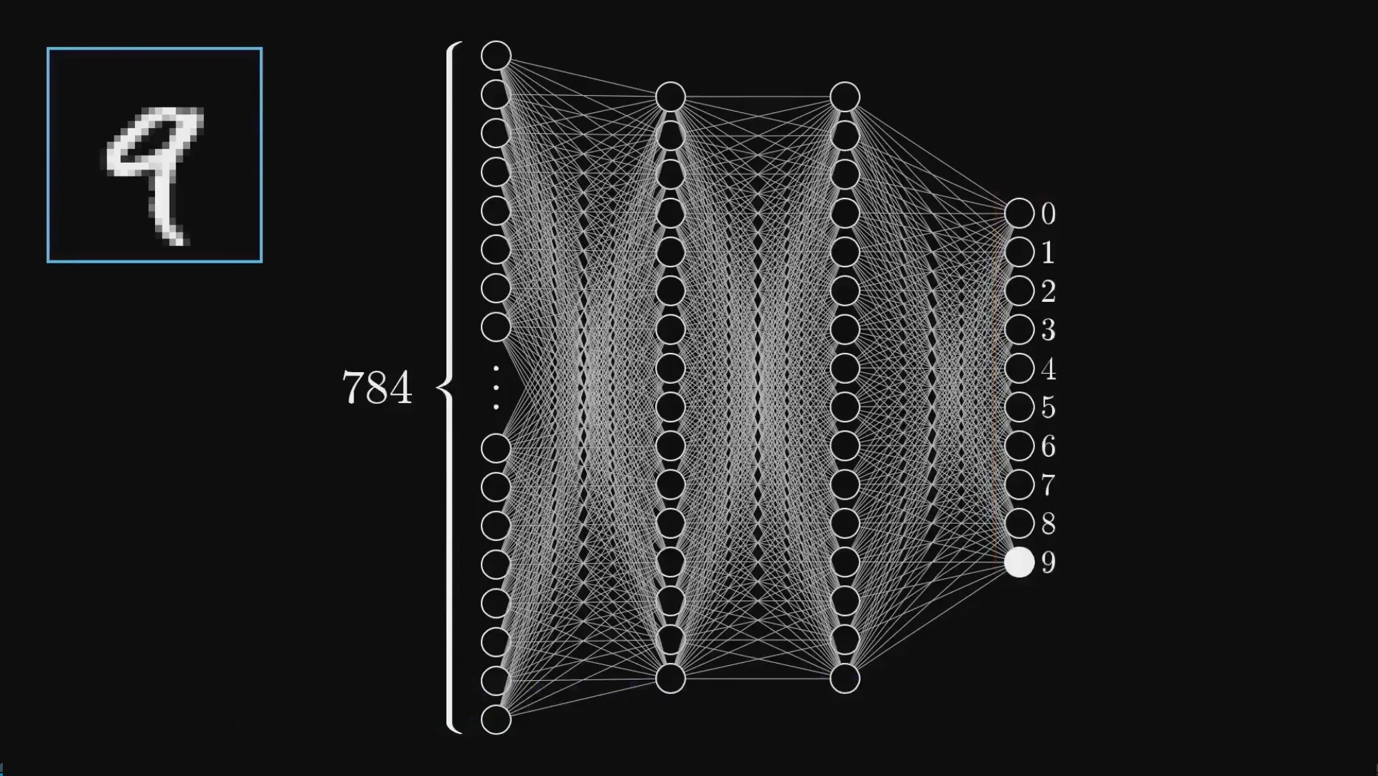
Why choose 2 hidden layers with 16 neurons each? No theoretical basis. This is purely for visual appeal and intuitive understanding. In practice, the number of hidden layers and neurons per layer are hyperparameters that need to be tuned experimentally.
The Motivation for Layers: Hierarchical Abstraction#
The core idea of hierarchical structure is to break complex problems into simpler subproblems, organized by spatial granularity:
pixels → small edges → larger parts → complete digitsTake recognizing the digit “9” as an example. Ideally, the first hidden layer detects an arc in the upper-right region and a vertical line on the right. The second hidden layer combines these two signals to recognize the pattern “circle on top + long vertical line on the right.” The output layer then lights up the neuron corresponding to digit 9 based on this combined pattern.
This is similar to the hierarchy in speech recognition: raw audio becomes phonemes, phonemes combine into syllables, and syllables form words. Each deeper level represents a higher level of abstraction.
But here’s an important note: this is only an intuitive expectation. As we’ll see later, a real trained network doesn’t work exactly this way.
Layer-to-Layer Transmission#
The value of each neuron in the next layer is determined by all neurons in the previous layer, computed as a weighted sum.
Let’s look at a concrete example. Suppose a neuron in the hidden layer is specifically designed to detect an edge pattern where “the middle is bright and the surroundings are dark.” The implementation is to assign positive weights (say +1) to pixels in the middle region, negative weights (say -0.5) to surrounding pixels, and 0 to the rest. When the input image happens to have a bright middle and dark surroundings at the corresponding location, the weighted sum reaches its maximum, and this neuron “lights up.” Each hidden layer neuron is essentially using its weights to describe an input pattern it cares about — conceptually identical to template matching with convolution kernels in image processing.
The weighted sum itself can be any real number, but two additional components are needed to form a complete computation.
The first is the bias. Bias controls how easily a neuron activates. If you don’t want the neuron to activate as soon as the weighted sum barely exceeds 0, but instead want it to only activate when a certain threshold is reached, you add a negative constant to the weighted sum. The more negative the bias, the more “picky” this neuron is — it needs stronger input signals to activate it.
The second is the activation function. It compresses the weighted sum (an arbitrary real number) into the range 0 to 1. The traditional choice is the Sigmoid function:
Very negative inputs give outputs close to 0, very large positive inputs give outputs close to 1, with a smooth transition zone around 0.
The complete computation for a neuron is:
In matrix form for the entire layer:
is the activation column vector of the previous layer (784-dimensional), is the weight matrix (16×784, each row corresponds to all weights for one neuron in the next layer), is the bias vector (16-dimensional), and is applied element-wise. Each layer is a matrix multiply plus a nonlinearity — the entire network is just nested compositions of this operation.
The Problem with Sigmoid and ReLU#
But Sigmoid is no longer used in modern deep networks.
The problem lies in the gradients. Sigmoid is almost completely flat at both ends — when the input is very large or very negative, the function curve is nearly horizontal. This means that making small adjustments in these regions barely changes the output. During later stages of training, many neurons’ inputs fall into these flat regions, and the backpropagated signal approaches zero as it passes through these positions, causing learning to stall. This phenomenon is called gradient saturation.
Modern networks use ReLU instead of Sigmoid:
Negative inputs directly output 0, positive inputs pass through unchanged. The form is extremely simple, but the gradient is always 1 on the positive half-axis, so it never saturates. Deep networks train much faster with ReLU than with Sigmoid.
Parameter Scale and “Network as Function”#
Let’s calculate the total number of adjustable parameters in our handwritten digit network:
| Connection | Weights | Biases |
|---|---|---|
| Input → Hidden 1 (784×16) | 12,544 | 16 |
| Hidden 1 → Hidden 2 (16×16) | 256 | 16 |
| Hidden 2 → Output (16×10) | 160 | 10 |
| Total | 12,960 | 42 |
That’s 13,002 adjustable parameters total. This is a very small network by deep learning standards, but sufficient for explaining core concepts.
The entire network is a function. It takes 784 numbers (pixel values) as input and outputs 10 numbers (confidence for each digit). Although the internal structure is complex with many parameters, conceptually it’s no different from — both take in a set of numbers and output a set of numbers. The difference is only in the number of parameters and depth of nesting.
“Learning” translated into mathematical language means: automatically finding the optimal combination of these 13,002 numbers from the training data.
The Learning Process of Parameters#
The Cost Function#
When a network is first initialized, all parameters are random. Feed it an image of “2,” and the 10 output neurons’ activations are all over the place — maybe 0.5, 0.8, 0.2, with no discernible pattern, nowhere near the ideal output (1 for the neuron corresponding to “2,” 0 for the rest).
To make the network learn, we first need a number that quantifies “how bad the current parameters are.” The simplest approach is to sum the squared errors for each output neuron:
is the actual value of the j-th neuron in the output layer, and is the expected value. If the network guesses correctly, this number is close to 0; if it’s wrong, the number is large.
Averaging this cost over all images in the training set gives us a function that takes 13,002 parameters as input and produces a single real number as output. This is called the cost function.
There’s a conceptual leap worth pausing to appreciate. The neural network itself is a function: 784 pixels → 10 numbers. The cost function is another layer of abstraction on top of that: 13,002 parameters → one number (describing how bad the network is). What you’re adjusting isn’t the network’s output directly, but this meta-function that describes the network’s quality. The entire meaning of “learning well” is to make this meta-function as small as possible.
Gradient Descent#
The problem becomes a purely mathematical optimization task: given a function of 13,002 variables, find the set of inputs that minimizes it.
Start with a simple case. If the cost function has only one parameter , you can plot the curve and find the valley bottom. The method: pick a starting point at random, compute the slope (derivative) at that point, move left if the slope is positive, move right if it’s negative, with step size proportional to the slope magnitude — take big steps when far from the valley, small steps when close.
Generalize to the case of 13,002 parameters. The cost function becomes a “hyper-surface” in 13,002-dimensional space. You can’t visualize it, but the core question remains the same: from the current position, in which direction should you take a step to make the cost decrease most quickly?
The answer is the negative gradient direction. The gradient is a 13,002-dimensional vector, and each component tells you two things: whether this parameter should increase or decrease (the sign), and how much changing this parameter contributes to reducing the cost (the absolute magnitude).
The update formula:
is the learning rate, controlling how big each step is. Too large and you’ll overshoot the valley and oscillate; too small and convergence is excruciatingly slow. Typical values are between 0.001 and 0.1.
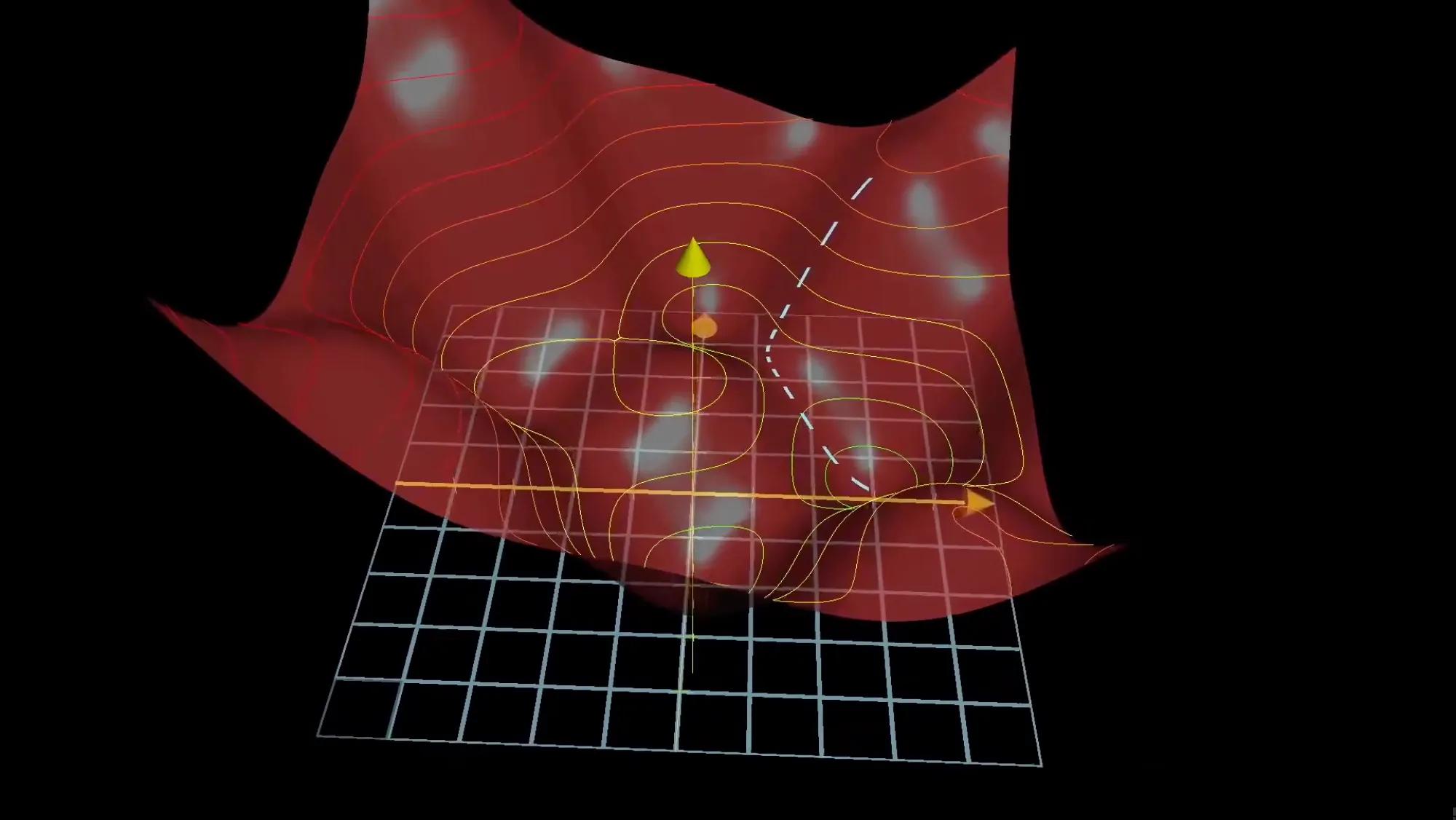
For a network with only two parameters, you can clearly see valleys and peaks on the cost surface in 3D space. Then extend this intuition of “walking in the steepest downward direction” to the unvisualizable 13,002 dimensions — using low-dimensional intuition to understand high-dimensional behavior is a key skill for understanding deep learning.
Physical analogy: You’re on a mountain ridge shrouded in fog, unable to see the surrounding terrain, only able to feel the tilt of the ground beneath your feet. You take a small step in the steepest downhill direction, stop to feel the tilt again, and take another step. You stop when you no longer feel any slope — this is a local minimum, but not necessarily the global one.
Surprising Findings After Training#
After training, this small network achieves about 96% accuracy on the test set. But one finding didn’t match expectations.
Remember the “ideal hierarchy” mentioned earlier? We expected the first layer to learn edge detectors, and the second layer to learn combinations of circles and lines. In reality, the second layer’s weights look almost random, with only faint directional patterns. The network did achieve 96% accuracy, but it didn’t follow the human-intuitive “edge → part → digit” path. In the 13,002-dimensional parameter space, it found a completely different location that also achieves a low cost.
An even more interesting phenomenon: feed this trained network pure random noise (not an image of any digit), and it will confidently classify the noise as some digit, say “5.” It won’t say “I don’t know.” The reason is simple — the cost function never required the network to have the ability to “doubt itself” during training. The training set only contains real handwritten digits; the network has never seen inputs that “aren’t digits,” so naturally it doesn’t know to output low confidence for such inputs.
Facts that keep recurring:
- Gradient descent only finds some local minimum, not necessarily the solution you intuitively expect
- The network will exploit any statistical clue in the training data, including ones you’re completely unaware of
On two controversial papers: The first paper scrambled all training labels (images unchanged, but labels became random values) and found that the network could still achieve the same accuracy on the training set — it was brute-force memorizing random data with millions of parameters. The second paper rebutted: although both cases eventually fit, the cost decreased extremely slowly (nearly linear) on random labels, while it decreased rapidly on real data. The conclusion is that the network does learn structure in the data, and structured data makes it easier to find good local minima.
Backpropagation#
The strategy of gradient descent is clear — walk in the negative gradient direction. But executing it requires efficiently computing 13,002 partial derivatives. Computing derivatives numerically for each parameter one by one requires O(n²) computation (where n is the number of parameters), which is completely infeasible for GPT-3 with 175 billion parameters. The backpropagation algorithm, through one forward pass and one backward pass, computes the gradients for all parameters in just O(n) time.
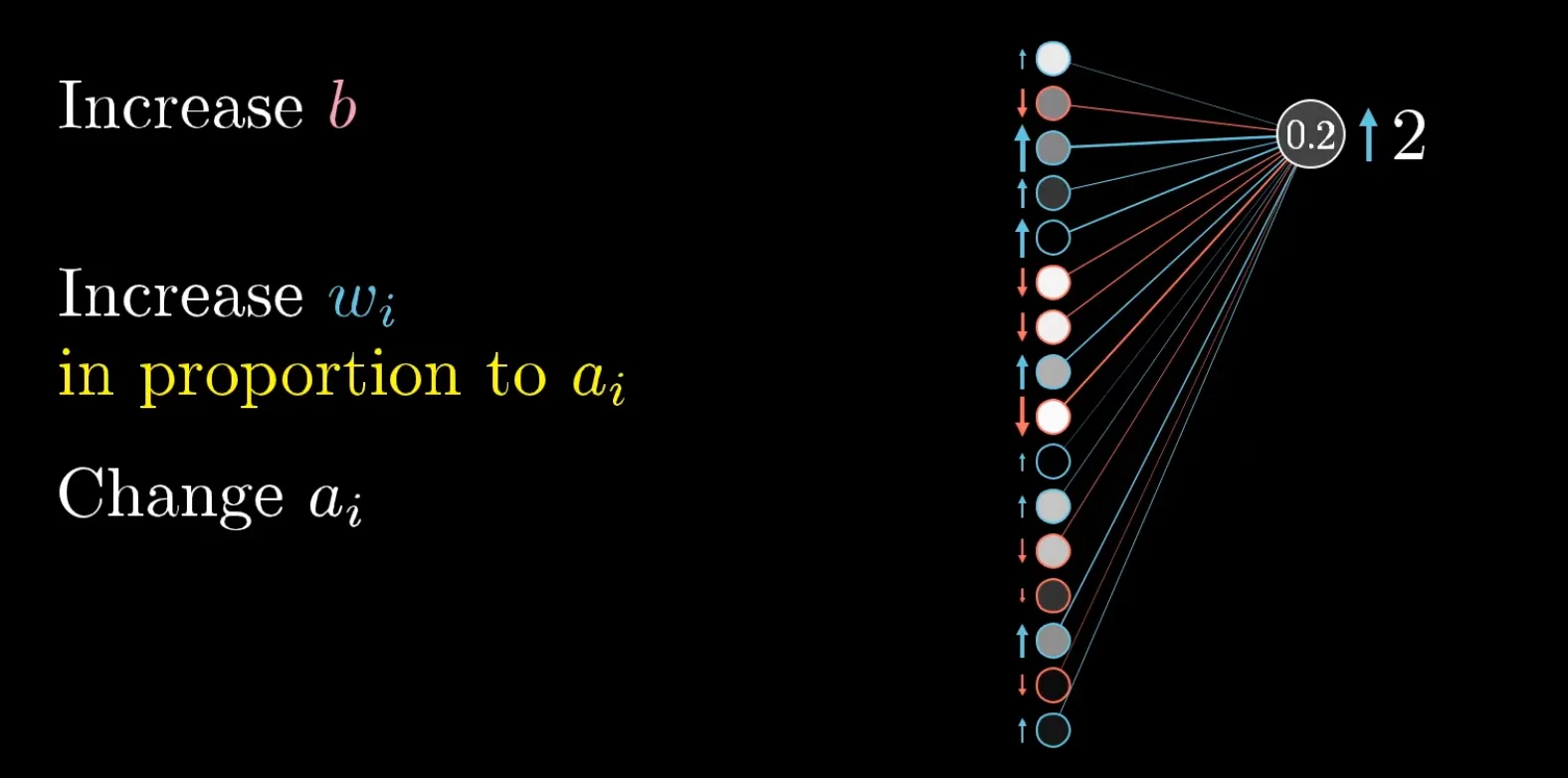
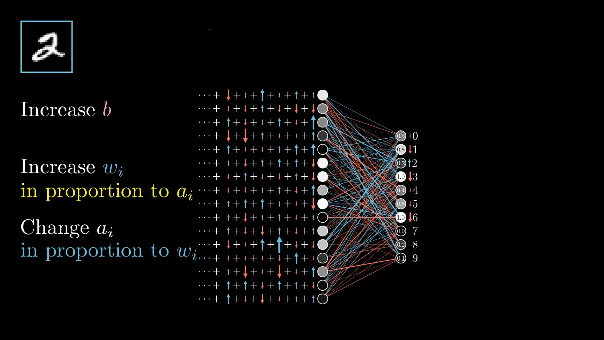
Feed an image of “2” into the network, and the current output is messy — the neuron representing “2” in the output layer isn’t bright enough. To make it brighter, there are three paths of adjustment:
First: Increase its bias. The most direct approach — larger bias means a larger weighted sum, which means a higher activation value.
Second: Increase its weights to the previous layer’s neurons. But there’s an efficiency issue here. The effect of adjustment is proportional to the current activation of the previous layer’s neuron. If an upstream neuron is currently near 0 (barely lit), even significantly increasing the weight connecting to it has negligible effect — because the weight multiplied by a near-zero number is still near zero. Conversely, if an upstream neuron is very bright (say 0.9), the same weight adjustment has a 9× greater impact. So the payoff of weight adjustment is proportional to the activity of the upstream neuron.
Third: Change the activation values of the previous layer itself. You can’t directly modify the activation values (they’re computed), but this leads to a core insight — you need to make upstream neurons that connect to the current neuron with positive weights brighter, and those connected with negative weights dimmer.
This is the manifestation of Hebbian theory in backpropagation: connections between simultaneously firing neurons should be strengthened (“Neurons that fire together, wire together”). If an upstream neuron is bright, and our goal is to make the current layer brighter too, then the weight between them should increase.
So far we’ve only discussed the desire of one output neuron. But the output layer has 10 neurons, each with its own adjustment demands on the second-to-last layer. These demands are weighted and summed — the “should you get brighter or dimmer” signal a particular upstream neuron receives is the sum of all downstream neurons’ demands. After the summation, the same logic is applied recursively to the earlier layer.
This is the origin of the name “backpropagation”: the dissatisfaction of the output layer is passed backward through the network layer by layer.
The Chain Rule#
To see the core logic, consider an extremely simple network — one neuron per layer, with only 3 weights and 3 biases total. Let the last layer’s activation be , and the cost for a single sample be .
To compute the partial derivative of the cost with respect to the last layer’s weight , the chain rule gives:
These three terms correspond to three cascading cause-and-effect relationships: tweaking first changes the weighted sum , the change in passes through the activation function to change , and the change in finally reflects in the cost . Like three interlocking gears — push the first, and the others follow.
Computing each term:
| Term | Result | Physical Meaning |
|---|---|---|
| Larger error means stronger adjustment | ||
| Slope of the activation function at the current position. If saturated (Sigmoid’s flat ends), this term is near zero and learning stalls | ||
| Activation of the previous layer. The brighter the previous layer, the more worthwhile it is to adjust this weight |
The product of these three terms is the complete gradient for a single weight:
The gradient for the bias is similar, but , so the term is absent.
When generalizing to real multi-layer, multi-neuron networks, the formula gains an extra pair of indices , but the structure remains identical. The only added complexity: a previous-layer neuron influences the cost through multiple paths (connected to multiple downstream neurons), so all the errors from downstream must be summed when propagating:
This summation is the entirety of backpropagation: the error of each downstream neuron, multiplied by the corresponding weight, accumulated back to the corresponding upstream neuron. Then the process recurses and continues forward.
The revolutionary aspect of backpropagation isn’t how clever the math is, but the complexity. Computing derivatives numerically for each parameter requires O(n²) cost; backpropagation only needs O(n) through one forward and one backward pass. The fact that GPT-3 with its 175 billion parameters can be trained at all depends on this fact.
From a broader perspective, a neural network can be viewed as a directed acyclic graph (computation graph), where each edge is a function dependency. Backpropagation traverses this graph backward from the root node (cost), computing each node only once to avoid redundant computation. This perspective is the core engine of modern deep learning frameworks (PyTorch, TensorFlow) — reverse-mode automatic differentiation. You don’t need to implement backpropagation yourself; the framework does it for you. But understanding the principle helps you know what’s happening when debugging and optimizing.
Stochastic Gradient Descent#
The theoretical version of gradient descent requires computing one gradient using all tens of thousands of images before making one update. At modern scales, this is completely unrealistic — GPT-3’s training set has hundreds of billions of tokens, and traversing all the data to compute a single gradient could take days.
Stochastic gradient descent (SGD) makes one change: use only a small batch of data (mini-batch, say 100 images) each time to estimate the gradient. This estimate is noisy — the direction of this small sample won’t be exactly the global steepest direction.
Why is noise actually a good thing?
Two people descending a mountain in thick fog. The first person stops at every step to precisely measure the steepest direction — the path is straight but every step takes forever to compute. The second person, slightly drunk, takes a rough guess at the direction and steps — the path is zigzagging, but each step is extremely fast, and they reach the bottom first as a whole. More importantly, the drunk’s zigzag path is less likely to get stuck in shallow ditches — those shallow valleys that would trap the precise walker are simply jumped over by the noise.
The randomness of SGD is a feature, not a bug. Noise gives the network a better chance of finding a truly good solution rather than getting stuck in the shallowest local minimum.
The Training Loop#
Putting everything together, one complete training iteration looks like this:
Initialize parameters (fully random)
    ↓
Loop:
    1. Take a mini-batch of data
    2. Forward pass: compute each neuron's activation layer by layer, get final output and cost
    3. Backward pass: starting from the output layer, compute gradients for each parameter layer by layer
    4. Parameter update: tweak all parameters in the negative gradient direction
5. Return to step 1 until the cost no longer decreases significantlyThroughout this process, backpropagation is the key to gradient descent. Without it, you can’t efficiently compute which direction each of the 13,002 parameters should be adjusted and by how much.
Embedding Vectors and High-Dimensional Space#
The discussion in the previous three sections was based on images — input that naturally comes as pixel values. But when it comes to text, the first question is: how do you turn words into vectors? And not just random IDs, but vectors that can express semantic relationships in geometric space.
Word2Vec: Learning Vectors from a Word-Guessing Game#
Nobody sat down and manually annotated that “king” should have coordinates [0.12, -0.34, 0.67…]. All the dimensions of embedding vectors are automatically learned from an extremely simple task: guessing words.
Take Word2Vec’s training approach as an example. Read through massive amounts of text — Wikipedia, news, books — and go through each sentence, each time removing one word and having the model guess it. In the sentence “The ___ sat on the throne ruling the nation,” the model needs to pick the most likely word from the vocabulary (tens of thousands of words) to fill the blank. This is essentially a multi-class classification problem.
Here’s how the training works. Initially, each word is assigned a random vector (say 300 dimensions). At this point, “king” and “apple” are about the same distance apart in space — no semantics at all.
Then the guessing begins. The model sees the context “sat,” “on,” “the,” “throne,” “ruling,” “the,” “nation” and predicts what word should be in the blank based on their current vectors. There’s a gap between the prediction and the correct answer (“queen”), the error is computed, and backpropagation simultaneously adjusts two things: the vector coordinates of relevant words in the embedding matrix, and the classifier parameters.
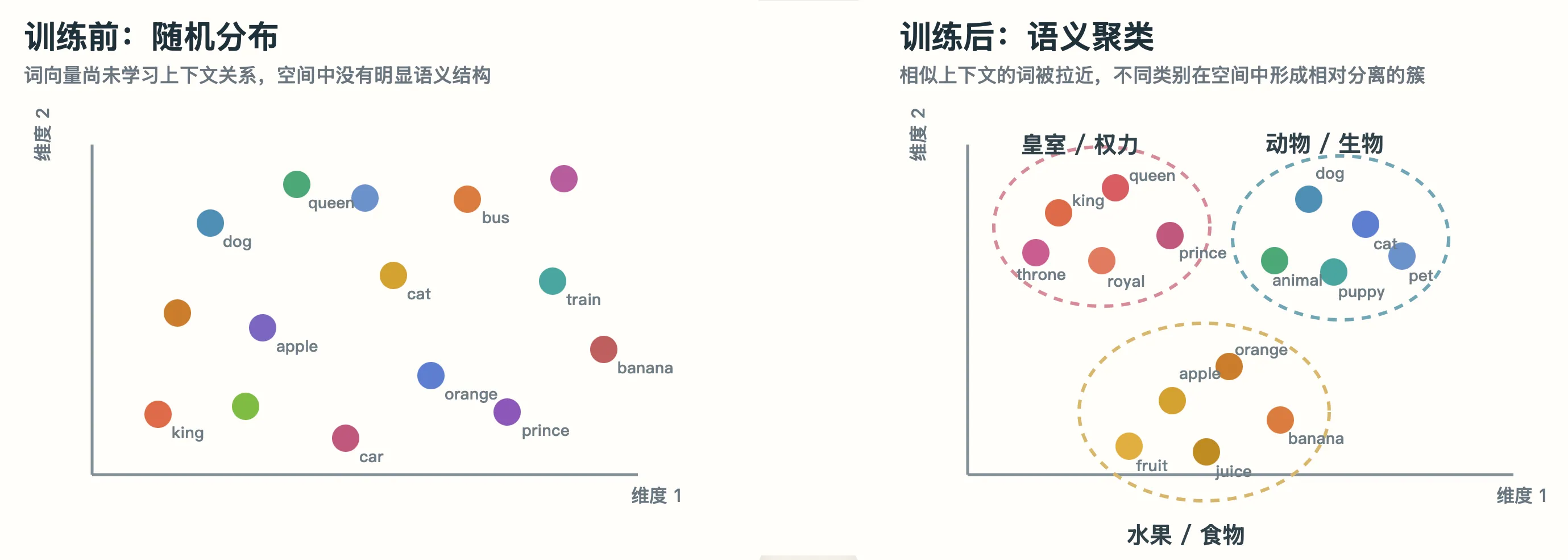
Every time it sees a sentence like “the king rules the nation,” it pushes the vector for “king” a bit toward the context words “rules” and “nation.” After billions of such guesses, words that frequently appear in similar contexts naturally end up close together. “King” and “queen” are surrounded by “prince,” “throne,” “rule,” “royal” — they’ve been pushed into a semantic cluster by their shared contexts.
Let’s illustrate this process with a simplified 2D space:
Before training (random):
    king·        ·apple
         ·queen
    ·man
              ·car
         ·woman

After training (billions of guesses):
    king·  ·queen
    man·  ·woman

    apple·  ·banana

car· ·truckSemantically similar words have clustered together. And directions have begun to encode relationships: the arrow “king → queen” ≈ the arrow “man → woman” (this direction encodes “femininity”).
The Distributional Hypothesis#
The process above has a linguistic theoretical foundation. The distributional hypothesis, proposed by J.R. Firth in 1957, can be condensed into a single sentence: “You shall know a word by the company it keeps.”
If two words frequently appear in similar contexts, their meanings must be close. “Apple” and “banana” both appear with “eat,” “fruit,” and “sweet”; “car” and “truck” both appear with “drive,” “road,” and “transport.” Word2Vec simply turns this linguistic principle into an optimizable mathematical objective — through gradient descent, the model gets better and better at the word-guessing task, and the semantic structure of the embedding vectors emerges as a byproduct of this optimization process.
Directions Encode Semantics#
Trained embedding spaces exhibit a surprising regularity: a particular direction in the space can encode a specific semantic relationship. The classic example:
"" points in the direction of “femininity” in the embedding space. Moving the “king” vector in this direction lands it near “queen.”
The same directional logic spans the entire vocabulary: Italy - Germany + Hitler is close to Mussolini; Germany - Japan + sushi is close to German sausage.
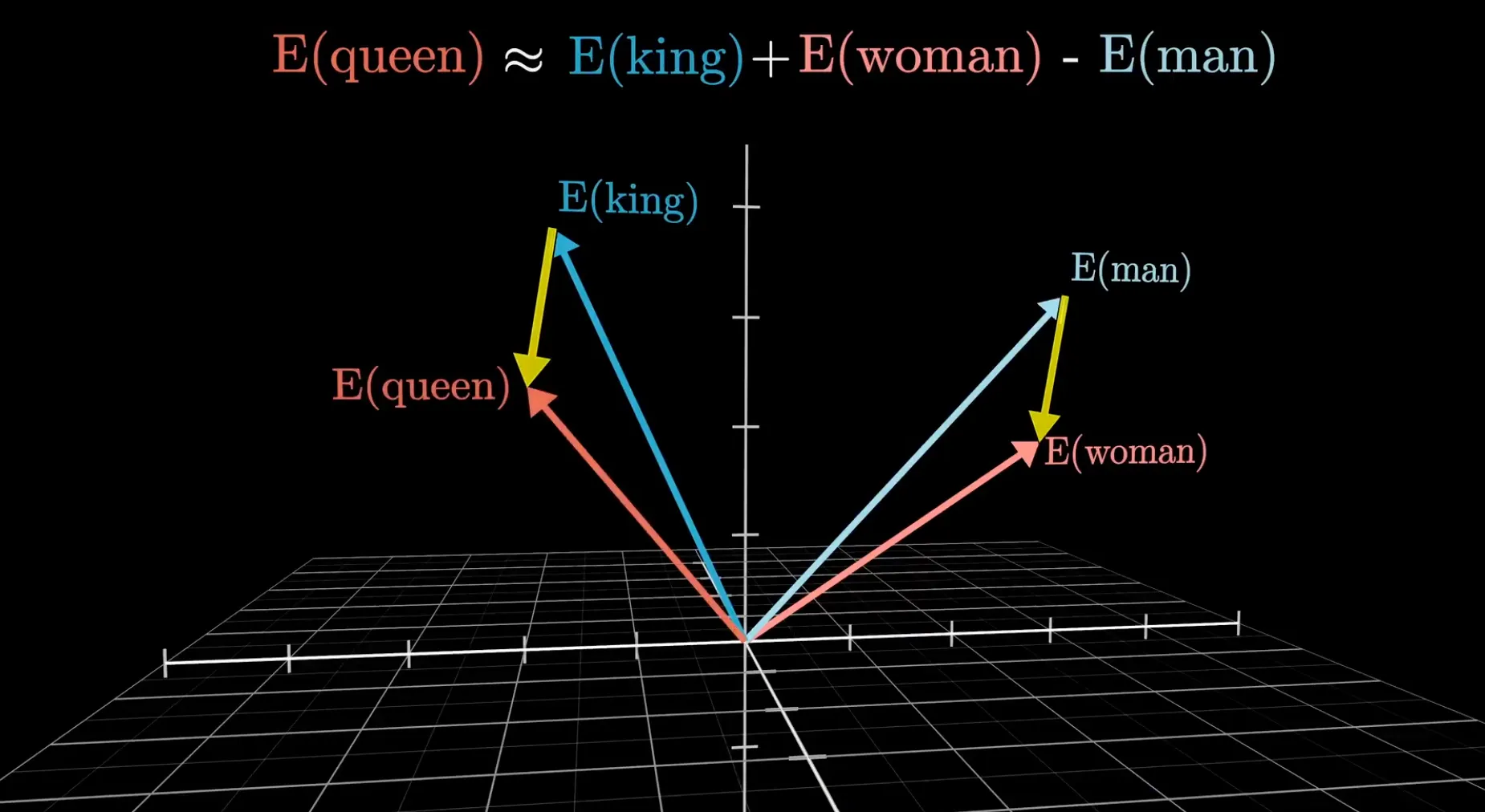
Why does this regularity emerge? Because the model discovered during training that arranging the relationship between “country” and “well-known X of that country” as a consistent displacement vector results in the best performance on the word-guessing task. There’s no deep philosophy behind this — the consistent displacement of analogical relationships happens to be the most compressed, most efficient representation of textual data. There’s no mathematical reason it had to appear, but the regularities in the data forced it to.
More concretely, the model is trained to predict that “when France appears, Paris is likely to appear nearby.” To make this prediction accurate, the model must place “France” and “Paris” in positions that express this relationship. Similarly, “UK” and “London” must satisfy a similar relationship. The end result is that the displacement vector “France → Paris” ≈ “UK → London” — this direction is the “capital relationship vector” in the embedding space. The positional relationships are a natural result of training, not artificially imposed.
Geometric Intuition of High-Dimensional Space#
In GPT-3, each word vector is 12,288-dimensional. At first glance this seems absurd — does understanding human language require 12,288 axes?
The role of dimensionality isn’t about the number itself. High-dimensional space has a counterintuitive geometric property: two randomly chosen high-dimensional vectors are almost certainly nearly orthogonal.
In 3D space, the angle between two random vectors is uniformly distributed between 0° and 180° — any angle is possible. But in 12,288 dimensions, the angle between any two randomly drawn vectors is almost certainly between 89° and 91°. Nearly perfectly orthogonal.
This means you can safely place the “basketball direction” and the “car direction” in the same 12,288-dimensional space, and they naturally won’t interfere with each other. You don’t need to carefully select 12,288 strictly orthogonal coordinate axes — high-dimensional space itself is composed of countless nearly orthogonal free directions.
A more precise mathematical description comes from the Johnson-Lindenstrauss Lemma: in high-dimensional spaces, allowing directions to deviate slightly from orthogonality (89°~91°), the number of approximately independent directions you can fit grows exponentially with dimension.
3Blue1Brown verified this conclusion with a Python simulation. Starting from 10,000 random 100-dimensional vectors, he pushed all pairwise angles into the 89°~91° range through simple optimization. 100 dimensions can accommodate 10,000 nearly independent conceptual directions. How many can 12,288 dimensions hold? Exponentially more.
This explains how language models can store an astronomical number of semantic concepts in a finite number of dimensions. The number of concepts stored in the model far exceeds 12,288 — they’re distributed across different nearly independent directions, with minimal mutual interference.
But this comes at a cost: individual features aren’t encoded by single neurons but are distributed across the joint activation patterns of groups of neurons. This phenomenon is called superposition. You can’t say “neuron #42 represents basketball” — in reality, hundreds of neurons collectively encode the concept of basketball. This is why neural network interpretability is so difficult. Anthropic’s sparse autoencoder research direction is an attempt to “unravel” these superimposed features.
Additionally, high-dimensional space has another benefit: linear separability is greatly enhanced. On a 2D plane, separating red and blue points might require a complex curved boundary. But in high-dimensional space, almost any classification pattern can be separated by a hyperplane (a simple linear split). The model doesn’t need complex nonlinear structures to determine “which words belong to sports” — a simple direction plus a threshold suffices.
Positional Encoding#
Vectors retrieved from the embedding matrix only contain semantic information. The vector for “Jordan” from the lookup table knows it’s a common surname, but it doesn’t know whether it’s in the subject or object position in the sentence, whether it follows “Michael” or appears at the end of the sentence. Positional information needs to be encoded separately.
The earliest positional encoding used fixed patterns of sine and cosine functions — each dimension encoded position indices with sine waves of different frequencies. The GPT series switched to learnable positional encodings: treated as another matrix that needs to be trained, optimized by gradient descent along with the embedding matrix during the word-guessing task.
The final input vector = embedding coordinates + position coordinates. The two layers of information — word meaning and word order — are combined and encoded before entering the first Transformer layer.
Transformer Architecture#
The Shortcomings of Fully Connected Networks for Text#
A fully connected network — with fixed 784 input pixels and 10 output digits — handles fixed-size images just fine. But text is completely different.
First, input length is variable. A sentence could be 3 words or 300 words. Second, language has directionality — in generation tasks, later words shouldn’t influence earlier ones. Most importantly, to accurately predict the next word, you need information from all previous tokens to converge at the last position, rather than each token producing independent outputs.
Before 2017, this problem was solved by RNNs and LSTMs with a “pass hidden state token by token” serial approach. Each time step processes one token and passes the current state to the next step. This works for shallow networks and short sequences, but for long sequences, the signal decays significantly as it’s passed token by token. And the serial computation completely fails to leverage the massive parallelism of GPUs — you have to wait for the first token to finish processing before you can start on the second.
The 2017 paper “Attention Is All You Need” introduced the core change: process all tokens simultaneously, with tokens communicating directly via dot-product matching rather than serial passing.
What GPT Means#
The three letters of GPT spell out its entire design intent:
- Generative: The model’s only output is the next likely token, which is then appended and used to predict further
- Pre-trained: All parameters have already been trained on massive amounts of text, ready for direct use or fine-tuning
- Transformer: The entire architecture is based on self-attention
As ChatGPT produces its output word by word, each step does exactly the same thing: take all the text currently available as input, output the probabilities for each of the 50,257 tokens in the vocabulary, pick one according to some strategy, append it to the input, and proceed to the next step.
Key constraint: when predicting the next token, the model can only see the text currently available, not “future” tokens. This constraint is enforced by the causal mask, which we’ll discuss later.
The Four-Stage Pipeline#
Data goes through four stages from input text to final output:
Stage 1: Tokenization + Embedding. Text is split into tokens (GPT-3 vocabulary size is 50,257, using BPE byte pair encoding that splits rare words into subwords). Each token looks up the embedding table to get a 12,288-dimensional initial vector, then positional encoding is added. The same word “mole” gets an identical initial vector regardless of context — contextual information is injected later by the Transformer blocks.
Stage 2: Transformer Block Loop. Vectors pass through attention layers and MLP layers in sequence. After each block, the vector coordinates are updated. GPT-3 repeats this 96 times.
Stage 3: Unembedding. Take the final 12,288-dimensional vector of the last token after 96 layers of modification, multiply it by the unembedding matrix (12,288 × 50,257), and get a 50,257-dimensional vector of raw scores (logits).
Stage 4: Softmax Sampling. Compress the 50,257 scores into a probability distribution, adjust the sharpness of the distribution with a temperature parameter, then sample to get one token.
Softmax and Temperature#
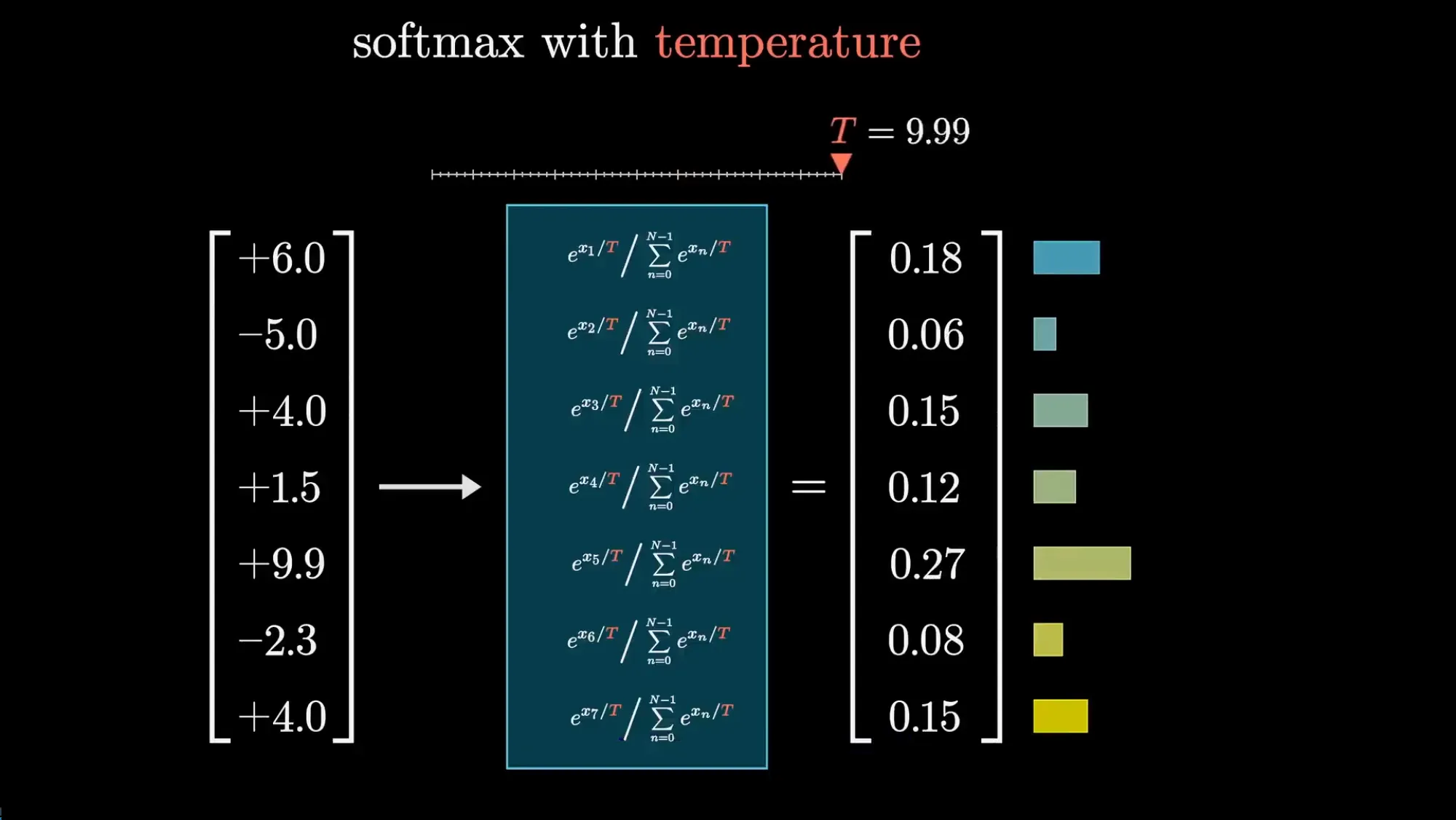
Softmax turns a set of arbitrary real numbers into a probability distribution: take for each number (making them all positive), then divide by the sum (normalizing to sum to 1).
The temperature parameter T works by dividing each score by T before taking the exponent:
- T→0: Only the highest-scoring token gets any probability, output is extremely conservative and repetitive
- T=1: Standard Softmax
- T>1: Distribution is flattened, the model is more willing to pick “less likely” words, output is more random
Use low temperature for code generation (high determinism), high temperature for poetry (more creativity). At T=2 or above, the output is essentially nonsense.
Attention Mechanisms#
The Polysemy Problem#
Returning to the issue mentioned in the embedding section. The word mole has the same initial embedding vector, but in three different contexts it expresses three completely different meanings:
American shrew mole— a small burrowing animalone mole of CO₂— a unit of measurement in chemistrybiopsy of the mole— a skin lesion
The initial embedding contains no contextual information — it’s just a fixed coordinate from a table lookup. The attention mechanism allows mole’s embedding vector to absorb information from surrounding tokens and shift toward the corresponding semantic direction. After absorbing information from CO₂, it moves away from its initial coordinates toward the chemical measurement direction; after absorbing biopsy, it shifts toward the dermatological direction. The same initial token, after different attention processes, becomes different vectors.
Query, Key, Value#
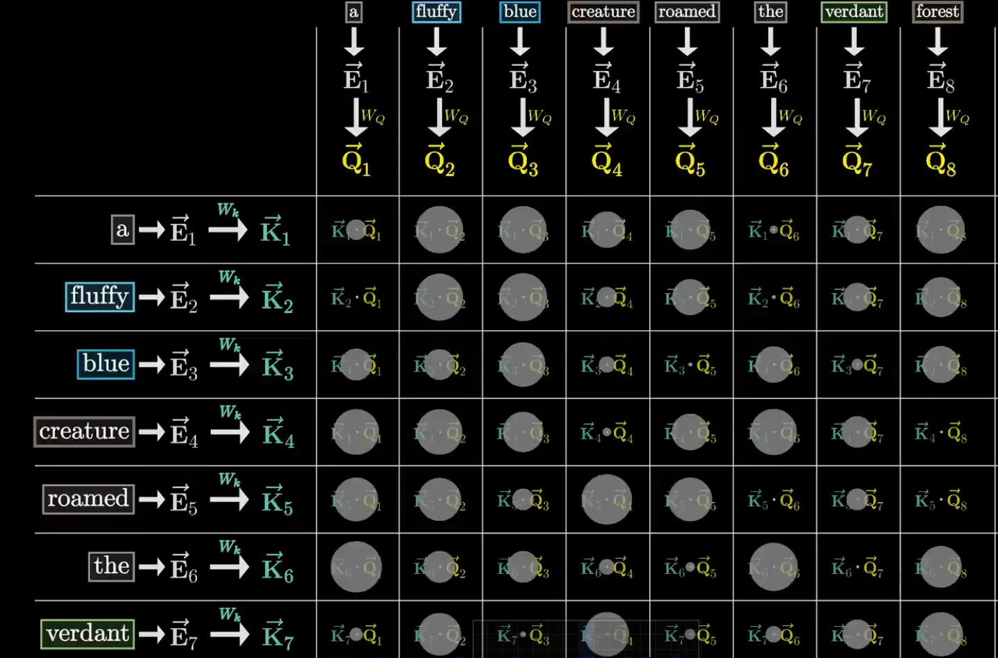
The core of the attention mechanism can be understood as a miniature retrieval system embedded within the Transformer. Using the sentence A fluffy blue creature roamed the verdant forest as an example. We want creature to absorb information from fluffy and blue — it needs to know it’s a “fluffy blue creature.”
Query is emitted by creature. It’s computed by multiplying creature’s 12,288-dimensional embedding by a learned matrix (128 × 12,288), compressing it to 128 dimensions:
Why compress to 128 dimensions? Because the Query’s job is just “matching” — extracting enough key features to determine relevance, without carrying the full 12,288 dimensions of information. It’s like entering only keywords when searching in a library, not the entire book’s content.
Key is generated by every token (including creature itself). Also computed from the 12,288-dimensional embedding via a learned (128 × 12,288) to produce a 128-dimensional vector:
Query and Key exist in the same 128-dimensional space — their dot product is the match score. creature’s Query dot product with fluffy’s Key is large (adjective→noun match is strong), with blue’s Key is also large, but with the’s Key is near zero (articles don’t carry much useful information for nouns).
Computing Query-Key dot products for all pairs of tokens gives an n×n grid (n is the context length). Then Softmax normalization is applied to each column (after dividing by to prevent numerical overflow), yielding attention weights that sum to 1 for each column.
Causal Mask#
During training, the model simultaneously predicts the next token after each position. If creature could “see” the words after it, it could know the answer in advance — that’s cheating.
The solution is to set the upper triangular region of the attention grid to before Softmax. After Softmax, these positions are precisely zero. The effect is:
     token1  token2  token3  token4
token1 [  ✓     -∞     -∞     -∞ ]  ← token1 can only see itself
token2 [  ✓      ✓     -∞     -∞ ]  ← token2 can see token1 and itself
token3 [  ✓      ✓      ✓     -∞ ]  ← token3 can see the first 3
token4 [ ✓ ✓ ✓ ✓ ] ← token4 can see allTokens at later positions cannot influence tokens at earlier positions at all. GPT-series models (Decoder-only architecture) always use causal masking — it’s a key mechanism for autoregressive generation.
Value and Embedding Update#
Query and Key determine “who should influence whom.” The content actually transmitted is in the Value.
Value matrix maps each embedding to a 12,288-dimensional vector — in the same high-dimensional space as the embeddings, so it can be directly used as a coordinate offset.
Weighted summing each token’s Value vector by the attention weights gives — the change to be added to the original embedding:
creature’s original coordinate has been pushed to a new position — it’s now not just a noun, but carries the information “fluffy, blue.”
The entire process, written in compact matrix form, is the famous formula from the paper:
Four operations: matrix multiply → divide by → Softmax → matrix multiply V. The output for each token is a weighted average of the Value vectors, with weights determined by Query-Key match scores.
Low-rank decomposition of the Value matrix
A naive would need to be a 12,288 × 12,288 square matrix — about 150 million parameters, far larger than Q and K’s ~1.57 million each (12,288×128). To balance parameter distribution, is decomposed into two smaller matrices multiplied together: (12,288×128) and (128×12,288), totaling about 3.15 million parameters.
This way, Q, K, V↓, V↑ are roughly the same size, with a single attention head having about 6.3 million parameters. This low-rank decomposition approach later inspired parameter-efficient fine-tuning methods like LoRA.
Multi-Head Attention#
A single attention head can only learn one type of relational pattern. It might be good at adjective→noun matching, or subject→verb matching, but it can’t handle all the different types of relationships simultaneously.
GPT-3 runs 96 independent attention heads in each layer. Each head has its own , , matrices, producing its own proposal. The 96 vectors are added together and then summed with the original embedding:
Head 1 → ΔE₁
Head 2 → ΔE₂
...
Head 96 → ΔE₉₆
        ↓
ΔE_total = ΔE₁ + ΔE₂ + ... + ΔE₉₆
        ↓
New embedding = Original embedding + ΔE_totalDifferent heads naturally differentiate into different attention patterns during training — some specialize in capturing grammatical relationships between adjacent words, some track long-distance anaphora resolution (e.g., “they” referring to “the researchers” 50 tokens earlier), and some handle more abstract semantic correspondences. Nobody arranges this division of labor in advance; it’s a stable configuration that gradient descent finds in the 175-billion-parameter space.
Parameter-wise: each attention head has ~6.3 million parameters, 96 heads × 96 layers ≈ ~58 billion parameters total for attention.
The size of the attention pattern matrix is n² (where n is the number of tokens). GPT-3 defaults to n=2048, corresponding to about 4 million elements. Extending the context to 128,000 tokens expands the grid to about 16.3 billion elements. Both computation and memory grow with n².
This is why long contexts are so difficult in engineering terms. Optimization algorithms like FlashAttention reduce memory overhead through block-wise computation, but the quadratic complexity of n² is an inherent cost of the attention mechanism.
Cross-Attention#
The GPT series uses only self-attention — both Query and Key come from the same set of tokens. But other architectures also include cross-attention:
| Type | Query Source | Key Source | Use Case |
|---|---|---|---|
| Self-Attention | Self | Self | GPT / Language models |
| Cross-Attention | Target language | Source language | Machine translation |
| Cross-Attention | Text | Image | Multimodal models |
Cross-attention is more commonly used in Encoder-Decoder architectures (translation models, image captioning models). GPT, as a Decoder-only architecture, doesn’t need it.
MLP and Fact Storage#
Where Are Facts Stored#
In December 2023, Google DeepMind published research on knowledge localization in LLMs, with a key finding: factual knowledge is primarily stored in the MLP layers, not the attention layers.
The division of labor is clear: Attention layers handle routing — they determine how information flows between tokens (“who should influence whom”). MLP layers handle content — they add solidified knowledge to the attention-modified vector coordinates (“what I know”).
The internal structure of a complete Transformer block is:
Input → [LayerNorm → Multi-Head Attention → Residual Connection]
      → [LayerNorm → MLP → Residual Connection]
→ OutputMLP processes each token’s vector independently (no communication between tokens at this step), but every token runs through the exact same MLP.
MLP Computation#
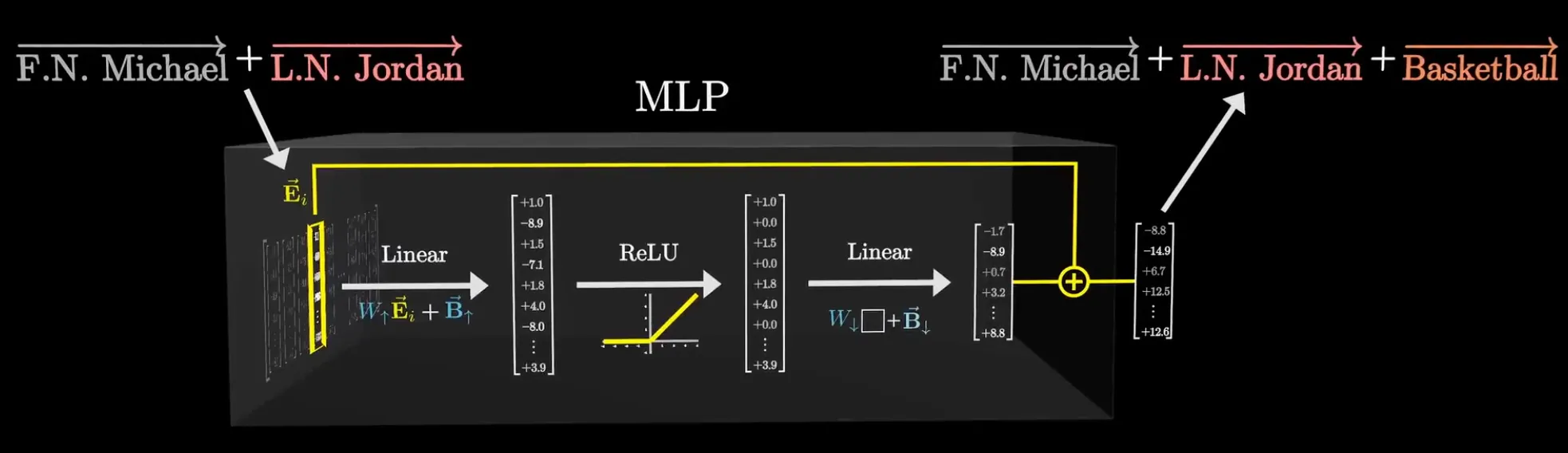
Let’s walk through the process with a concrete example. Assume there are three nearly orthogonal directions in the embedding space: encodes “first name is Michael,” encodes “last name is Jordan,” and encodes “basketball.”
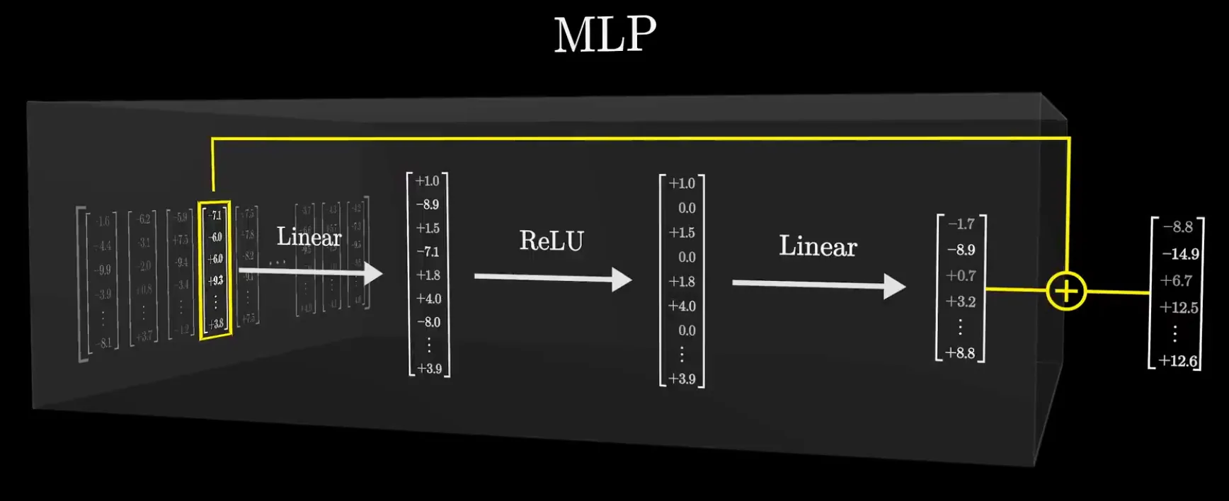
Step 1: Up-projection. Multiply the 12,288-dimensional input vector by (49,152 × 12,288), mapping it to a 49,152-dimensional intermediate space.
Each row of can be thought of as a “question vector” — it asks the input vector a specific yes/no question. For example, one row has been trained to be a combination like , asking “does this vector simultaneously carry components in both the Michael and Jordan directions?” With a bias of -1.5.
For the “Michael Jordan” embedding: dot product = 1 + 1 - 1.5 = 0.5 (positive). For other people’s embeddings: dot product ≤ -0.5 (negative).
In GPT-3, is 49,152 × 12,288 ≈ 604 million parameters. This is one of the largest single matrices in the entire network, second only to the embedding.
Step 2: ReLU (or GELU). All negative values are truncated to zero, positive values remain unchanged.
Its actual function is to implement an AND gate. Back to the Michael Jordan example: if and only if the input vector has sufficiently large components in both the and directions (weighted sum > 0) does this neuron output a positive value and pass the signal forward. If only one condition is met (e.g., Michael without Jordan), the weighted sum is negative, ReLU truncates it to 0, and the signal is blocked.
This is why nonlinearity is crucial in networks. Without it, multiple layers of matrix multiplication combine into a single linear transformation — the network couldn’t even express XOR. With ReLU, the network can make binary yes/no judgments on arbitrarily complex combinations of features in high-dimensional space.
Modern models commonly use GELU (a smooth version of ReLU), but the principle is the same.
Step 3: Down-projection. The activated 49,152-dimensional vector is multiplied by (12,288 × 49,152), bringing it back to 12,288 dimensions.
Each column of is a specific direction in the embedding space. If the first column corresponds to (the basketball direction), and the corresponding neuron was activated in step 2 (positive output), then the “basketball direction” is added back to the result vector. Other columns might encode related directions like “Chicago Bulls,” “jersey #23,” “shooting guard,” etc.
is also ~604 million parameters. A single MLP layer uses ~1.2 billion parameters to implement “conditional judgment + knowledge write-back.”
Step 4: Residual Connection. Output = Input + result from step 3. The input vector remains intact, and the MLP’s detection result is added to the original vector as an increment.
After 96 layers of such accumulation, the “Jordan” vector, which started as merely a surname, has layer after layer of MLP adding directional components like “plays basketball,” “American athlete,” “born in Brooklyn,” “1984 NBA draft,” eventually becoming a vector carrying a wealth of structured factual knowledge.
Parameter Statistics#
| Component | Parameter Count | Percentage | Role |
|---|---|---|---|
| Embedding Matrix | 617M | <1% | Turn tokens into vectors |
| Unembedding Matrix | 617M | <1% | Turn vectors back into tokens |
| Attention (96 layers × 96 heads) | ~58B | ~33% | Inter-token communication routing |
| MLP (96 layers) | ~116B | ~66% | Factual knowledge storage |
| LayerNorm etc. | ~3M | Negligible | Numerical stability |
| Total | ~175B |
Attention provides communication, MLP provides knowledge. MLP accounts for 2/3 of the total parameters — because storing facts requires far more parameters than routing information.
One Inference#
Asking “What Sport Does Michael Jordan Play”#
Given this input, here’s the complete process inside GPT-3:
Tokenization. The text is split into tokens: ["Michael", "Jordan", "plays", "what", "sport", "?"]. Each token has an ID in the vocabulary.
Embedding. Each token looks up the embedding table to get a 12,288-dimensional initial coordinate vector. “Jordan“‘s initial vector knows only that it’s a common surname — no information about basketball.
Add positional encoding. Position signals are added to each vector. “Jordan” is at position 2, “sport” is at position 5.
96 layers of Transformer processing. Each layer first runs attention (tokens exchange context), then runs MLP (adds detected facts to each vector).
In layer 1 attention, “Jordan“‘s Query matches “Michael“‘s Key strongly. “Jordan” absorbs a lot of information from “Michael,” moving its coordinates from “a common surname” toward “someone’s full name.” The attention layer doesn’t provide facts — at this point, “Jordan” doesn’t yet know it’s about basketball.
In layer 1 MLP, a row of detects the combination condition “simultaneously encoding Michael and Jordan directions” → ReLU activates → the corresponding column of adds the “basketball direction” to “Jordan“‘s vector. The initial “basketball” signal is injected.
In layer 2 attention, “Jordan“‘s coordinates now contain a “basketball” signal, so “sport“‘s Query match score with its Key increases — “sport” also begins absorbing the semantic bias toward “athletic competition.” Layer 2 MLP detects a richer feature combination and continues adding knowledge directions like “NBA,” “jersey #23,” etc.
The layer-by-layer refinement roughly follows:
| Layer Depth | What the Embedding Encodes |
|---|---|
| Shallow (1-10) | Grammatical relations: adjective→noun, subject-verb agreement |
| Middle (10-30) | Semantic relations: anaphora resolution, sentiment |
| Deep (30-96) | Abstract concepts: tone, style, scientific knowledge |
By the end of layer 96, the ”?” vector has absorbed, through attention, the most important information from the entire sentence — “someone named Michael Jordan, the question is asking about sport, and Jordan’s vector has a very strong basketball signal.”
Unembedding + Softmax. Take the final 12,288-dimensional vector of ”?”, multiply by the unembedding matrix to get 50,257 raw scores. “Basketball” scores far above all other words. After Softmax, its probability is about 89%. Sampling selects “basketball.”
Iterative generation. “Basketball” is appended to the input, and the entire process runs again — predicting the next word, then the next, until the model outputs an end token.
Input: "Michael Jordan plays what sport?"
        ↓
① Tokenize → ["Michael", "Jordan", "plays", "what", "sport", "?"]
        ↓
② Lookup embedding → each token gets a 12,288-dim initial coordinate
        ↓
③ Add positional encoding → coordinates carry positional info
        ↓
④ Enter 96-layer Transformer:
   ┌─────────────────────────────────────────┐
   │ Each layer does two things:              │
   │                                         │
   │  Attention layer: exchange context       │
   │    "Jordan"←→"Michael" (coordinate adj.) │
   │                                         │
   │  MLP layer: detect features + add facts  │
   │    Up-proj → detect "This is MJ"         │
   │    → ReLU gating                         │
   │    → Add "basketball" direction back     │
   │    → Residual preserves original info    │
   └─────────────────────────────────────────┘
        ↓
⑤ Take final coordinate of last token "?"
        ↓
⑥ Unembed → compute scores for each word in vocabulary
        ↓
⑦ Softmax → convert to probability distribution
        ↓
⑧ Sample → select "basketball"
        ↓
⑨ Append to input, repeat ①~⑧ → generate next word → until done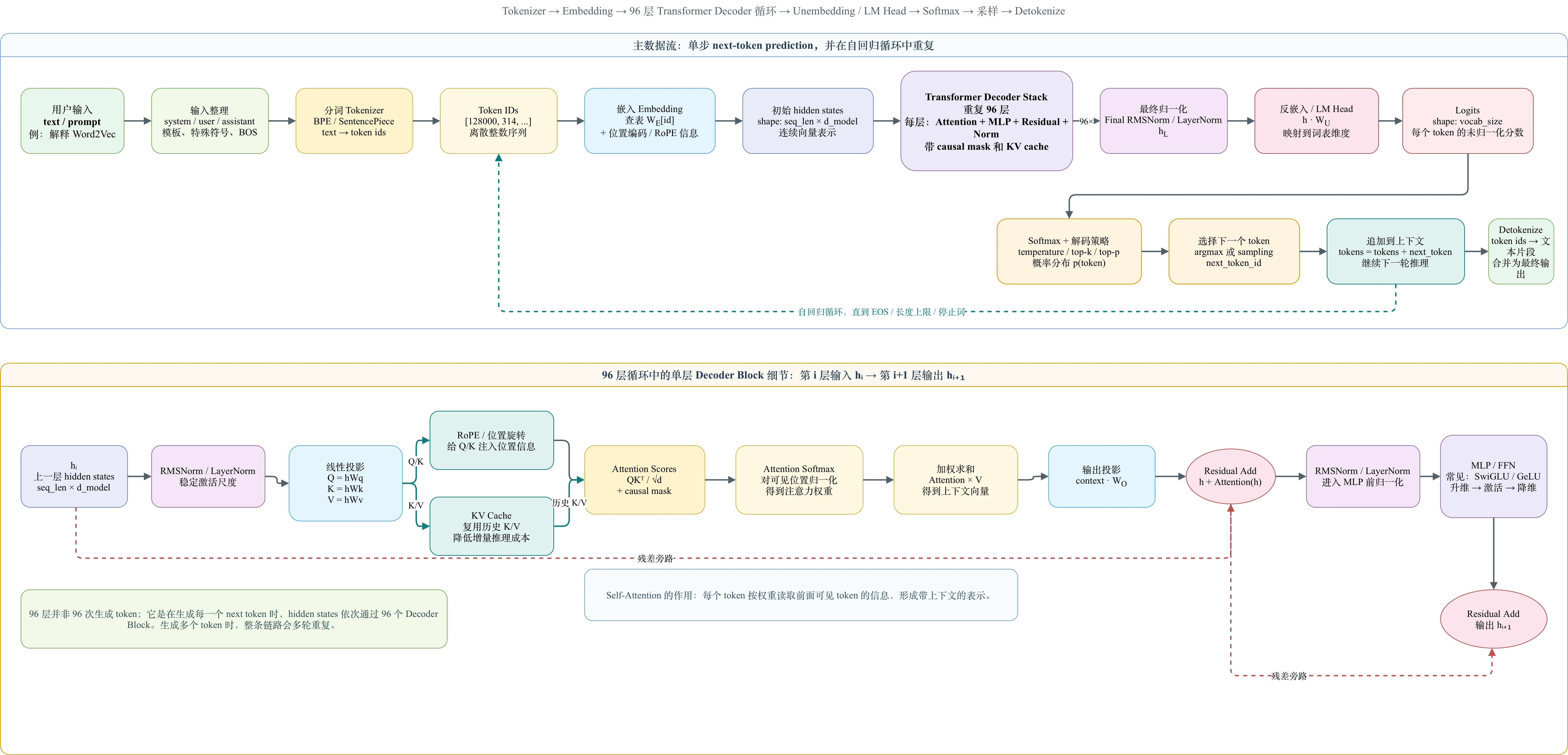
An Analogy#
Compare the entire Transformer process to 96 rounds of meetings at a company:
- At the start of each round, everyone first uses “attention” to hear the latest updates from others on the current topic, updating their own understanding
- Then each person consults their own professional database (MLP), writing relevant information found into their notes
- Notes use an append-only format (residual connections), not overwriting previous records — even if a particular round’s query goes wrong, earlier information is preserved
- After one round, the notes stabilize (LayerNorm), and the next round begins
After 96 rounds, each person’s understanding of the topic has evolved from vague fragments to a complete picture covering all relevant aspects. The last person (the last token)‘s notes contain the most comprehensive record of the entire meeting — output prediction relies on this final set of notes.
Auxiliary Components#
LayerNorm
Before each attention and MLP layer, normalize the vector values to have mean 0 and variance 1. Over 96 layers of continuous accumulation, without normalization, vector values would grow increasingly large or small, quickly leading to numerical overflow (NaN). LayerNorm ensures numerical stability in deep networks.
Residual Connection
Output of each layer = Input + the correction computed by this layer. Two core values:
First, original information is never overwritten. Even if a layer’s attention or MLP completely fails (outputs all zeros), the input information can flow unchanged to the next layer.
Second, gradients can “take a shortcut” from the output layer back to shallow layers, skipping intermediate layers. Deep networks without residual connections face the vanishing gradient problem — the error signal decays to nearly zero as it propagates layer by layer, and shallow layer parameters stop learning. Residual connections provide a gradient highway, allowing shallow layers to receive effective learning signals as well.
Embedding and Unembedding Parameter Sharing
In GPT-3, the embedding matrix and unembedding matrix typically share the same parameter set. The same mapping table handles translation in both directions: “token→vector” and “vector→token.” This imposes a strong constraint on the model: the representation for the same word must be consistent going in and coming out.
Further Reading#
What we’ve understood
- The training objective forces semantically similar words close together in high-dimensional space
- Directions can encode relationships — the displacement vector king→queen ≈ man→woman
- Attention enables information flow between tokens — “Jordan” can absorb context from “Michael”
- MLP stores and retrieves facts through up-projection + ReLU gating + down-projection write-back
- The near-orthogonal geometry of high-dimensional space provides exponential storage capacity
- Backpropagation makes O(n) gradient computation possible, enabling training of 175-billion-parameter models
What hasn’t been fully explained yet
- Why gradient descent consistently finds good local minima in such high-dimensional non-convex terrain without getting trapped by the vast number of saddle points. Existing theoretical directions (loss landscape connectivity) have made progress but can’t fully explain it.
- Why 12,288 dimensions is the practical sweet spot for GPT-3 — not so small as to limit expressiveness, not so large as to make training costs unbearable. This number is more the result of engineering experience and scaling experiments than first-principles derivation.
- What the activation patterns of middle and deep layer neurons are actually doing. This is what Anthropic’s Transformer Circuits team and the sparse autoencoder direction are actively researching.
- Why the model “automatically” aligns “king→queen” and “man→woman” in the same direction. We know the training objective makes this the most efficient representation, but why gradient descent reliably finds this structure rather than falling into some suboptimal, chaotic representation.
We know how it works, and we know how to make it work better, but at the granularity of “what features each neuron detects,” we’re still a considerable distance from complete understanding.
Extended Reading
- Andrej Karpathy — “Let’s build GPT from scratch”. Builds a GPT from zero, with clear explanations at every step. Good for those who want to get hands-on after reading this.
- “Attention Is All You Need” (Vaswani et al., 2017). The original Transformer paper. It’ll be much easier to read after understanding the above content.
- Christopher Olah’s Transformer Circuits blog series. Continuously updated on Anthropic’s website, currently the deepest work on Transformer interpretability.
- 3Blue1Brown’s deep learning video series. 3b1b’s animation is far more expressive than text, highly recommended to watch.